Second order tensors can be used to represent the state of stress and strain in
Lagrangian space or stress and strain rate in Eulerian space. Here a Lagrangian
approach is used where the components of any second order stress tensor can be
reduced to an eigenvalue problem and visualized as a quadric surface, Frederick
and Chang [9]. The components of a stress tensor can be written in a more
familiar matrix format where it is useful to show how each matrix term is a
vector component acting on the differential element shown in Fig. 27.
Figure 27. Stress tensor components shown on differential element.
When written in indical notation, σij, this second order tensor
obeys the transformation law, Eqn. (10), where aij is the rotational
transformation matrix. Not all matrices reduced to tensors. A quantity can
only be called a tensor if its components obey the tensor transformation law.
The term aij is the rotational transformation matrix defined in most
tensor theory text books. It is important to note that this transformation matrix
does not include translation as a fourth row and column, which is typically used
in most computer graphic software APIs (Application Programming Interfaces). In
the development that follows the relationship between this transformation matrix
and Euler angle will be used to rotate stress tensor glyphs into principal stress
states.
Here the second order stress tensor is transformed into an eigenvalue-eigenvector
problem using tensor notation instead of matrices because of its notational
brevity. For the reader who is more familiar with the matrix approach we leave
this as an exercise where the reader can refer to any standard text book on
deformable bodies.
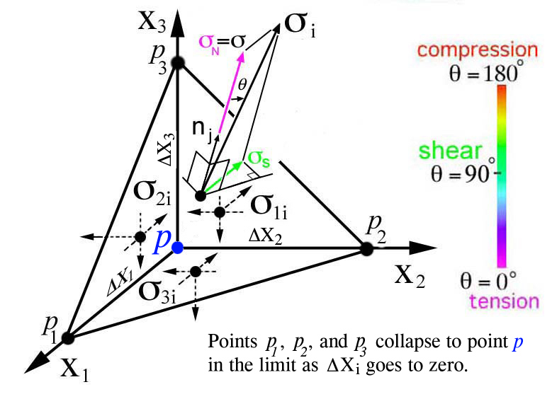
Stress can be represented both as a first order tensor, σi (vector),
and as a second order tensor, σij. These two types of stresses can
be related by cutting the differential element in Fig. 27 and applying a stress
vector on the cut plane (P1,P2,P3), Fig.
28. To maintain equilibrium the second order stress tensor components, shown on
the opposite facing surfaces as dashed lines, must be equal to the direction
cosine components of the first order stress tensor acting on the tilted plane
(P1,P2,P3). The orientation of the
tilted plane is arbitrary and defined by the direction cosines of the unit
normal vector, ni. Imagine that as the plane
(P1,P2,P3) is tilted, the magnitude and
direction of σi changes to maintain equilibrium with the second
order stress tensor components which are shown as dashed lines on the opposite
facing surfaces. Note the components of the second order stress tensor do not
change as the plane tilts. This equation should be called the equilibrium
equation, however to honor the accomplishments of a famous mathematician,
Augustin-Louis Cauchy (1789-1857), this relationship is called Cauchy's
equation (12).
In general σi and nj are oriented in different
directions and the first order stress tensor, σi, can be
resolved into normal and shear components, (σN,σS).
However the plane (P1,P2,P3) can be
oriented such that the first order stress tensor σi, and the
unit vector, nj, are parallel and the shear component goes to zero,
σS = 0. This special direction defines principal stress,
σ, when σS = 0. This principal stress can also be refered
to as σN, however traditionally the symbol σ is used in
the development of the eigen-value problem.
This special case is referred to as a principal direction where the magnitude of
this stress, σ, is called a principal stress, which is the scalar component
of σi projected onto the unit vector nj. The color
legend will prove useful when envisioning stress type as a color gradient
projected onto various stress glyph surfaces. Development of the eigen-value
problem continues using the principal stress, σ, without the use of color.
Equating Eqn.s (12) and (13) and rearranging indices on ni using the
Kronecker delta, δij, yields
The Kronecker delta, δij, is equivalent to the identity matrix.
Together with the orthogonality conditions there are four equations with four
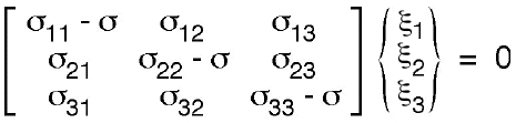
unknowns. Equation (15) becomes an eigenvalue problem which can be rewritten
here in a more familiar matrix notation,
where the stress scalars terms, σ, along the diagonal are the three
eigenvalues (principal stresses:
σa,σb,σc) and the column
vector are the eigenvectors (direction cosines: "orientations" of the
principal stress state). When the differential element shown in Fig. 27
is rotated into the principal stress state the normal stresses,
σxx, σyy, and σzz
become maximums and minimums
(σa,σb,σc) and the shear
stresses go to zero as shown on the cube to the right in Fig. 29.
This eigen-value problem is very common and there are numerous text books
on numerical methods that solve for the eigen-values and eigen-vectors. Here
the numerical solution is developed first followed by development of
customized stress tensor "glyphs" that will hopefully provide insight from a
scientific point of view. The development of the numerical solution follows.
Here a computer program is developed to solve for eigen-values and
eigen-vectors using a standard Jacobi method. The complete program (
eigen.f), sample data set (
sij.data), and corresponding results (
eigen-calc-details.out,
eigen-stress.out,
eigen-vectors.out) can be downloaded and used to reproduce
results shown here. Below we discuss the solution using code fragments.
The solutions assumes symmetric stress tensors therefore only six components
are read in the order shown in the code fragment below followed by the stress
location at coordinates x, y, and z. Here the notation for stress, s(i,j), is
setup as an array.
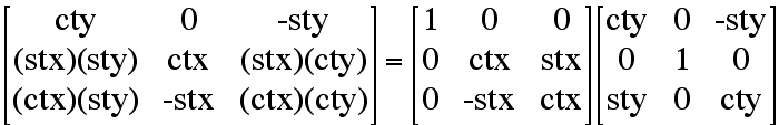
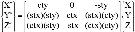
Given: aij, Find: Euler angles (θx,
θy, θz ). This is accomplished by creating a
transformation matrix, aij, from a sequence of three simple rotations
in Fig. 30. Because the rotation matrix, aij, is constructed from
Euler angle rotations, these angles can be extracted from this matrix using
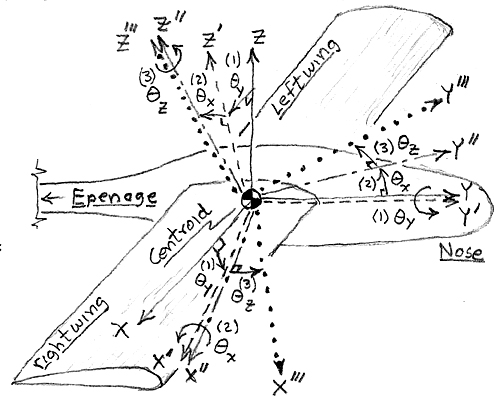
simple algebra. Here we use the same procedure and notation outlined by Bourke
[10]. The coordinate system shown in Fig. 30 is typically used in flight
simulators with the origin located at the aircraft centroid, with the y-axis
pointing forward, the x-axis off the right wing and the z-axis pointing up.
Rotation sequence is as follows: (1) "roll" positive to the right, (2) "pitch"
positive up, and (3) "yaw" positive to the left. Note: order matters, (1) ->
(2) -> (3) is not equal to (2) -> (1) -> (3).
Figure 30. Standard flight simulator coordinates and Euler angle rotations:
(1) roll, (2) pitch, (3) yaw.
Rotation sequence as experienced by a pilot sitting in the airplane cockpit,
Fig. 30: (1) roll right, +θy, Eqn. (17), (2) pitch up,
+θx, Eqn. (18), (3) yaw left, "heading", +θz,
Eqn. (19). In reverse order this orientation is known as heading-pitch-roll
(HPR).
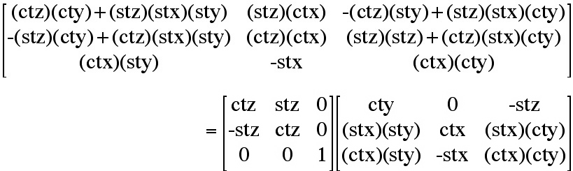
For brevity the following notation is used, for cosines: ctx=Cos(θx),
cty=Cos(θy), ctz=Cos(θz), and for sines: stx=
Sin(θx), sty=Sin(θy), stz=Sin(θz).
Combine roll followed by pitch.
Combine the roll and pitch transformation (20) above with the yaw transformation (19).
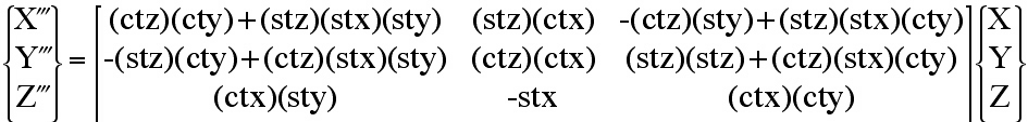
Combining all three transformations (1) -> (2) -> (3) yields the final transformation
Xi = aij Xj , where a11 = (ctz)(cty) +
(stz)(stx)(sty), a12 = (stz)(ctx), a13 = -(ctz)(sty) +
(stz)(stx)(cty), etc..
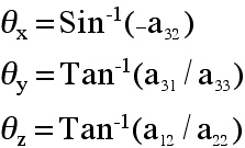
Recall notation -stx = -Sin(θx) = +a32 and collecting terms
a31/a33 and a12/a22, reduces terms to
a31/a33=[Cos(θx) Sin(θy)]/[
Cos(θx) Cos(θy)]=Tan(θy), and
a12/a22 =Tan(θz), which yields Euler angles as
functions of components of the transformation matrix, aij.
Recall the components of the transformation matrix, aij are equivalent
to the set of three eigen-vectors and can be used to calculate the Euler angles.
It is important to recall that the Eqn. (23) requires the rotation order,
θy, θx, θz be used when
implementing the rotation defined by the eigen-vectors orientation of the
principal stress state.
This completes the mathematical solution of the eigen-value solution of Eqn.
(16). Using these eigen-value and eigen-vector solutions, second order stress
tensor "glyphs" are developed next that emphasize different physical properties
of interest for the analysis of large data sets (insight) and for presentation
of results.
The eigen-value problem defined in Eqn. (16) appears frequently in the applied
sciences. Depending on the application the coefficient matrix consists of
different physical quantities. Although the mathematics provides a common
method for solving for the eigen-values and eigen-vectors, it is important to
maintian the physical context when creating a graphical representation (glyph)
of a physical property. It is often this context that leads to insight from the
scientists who are visualizing their complex data sets for the first time.
This is why the ESM4714 class is named "Scientific Visual Data Analysis" and
just not "Visualization" or "Information Visualization". To be insightful from
a scientific perspective the word scientific is used to qualify the type of
data analysis. This also explains why the development here continues with a
focus on the physical concepts of equilibrium and how the components of stress
are visualized as normal and shear componets that exist within the definition
of a stress quadric surface, e.g. stress tensor glyphs. Several researchers
[8,11,13,14] have demonstrated the usefulness of visualizing second order
tensor glyphs. The development of these glyphs revealed information that went
beyond the initial physical understanding of the problem. Similarly the
development of the glyph here also demonstrates how glyphs can provide insight
that transcends the traditional use of graphics, namely: graphics for
presentation. In the final section these ideas are extended to higher order
tensors. Through out the development of tensor glyphs shown here, the
quantitative mathematical idea of invariance of tensor equations is used to
qualitatively envision and understand physical properties and their
relationships as laws. Consequently envisioning invariance enables scientists
to see and understand the qualitative content of equations associated with the
physical laws, e.g. static equlibrium and dynamic equations of motion.
The development of the eigen-value problem requires that all properties and
their relationships exist at points. For example in Fig. 28 points P1
, P2, and P3 collapse to point
P in the limit as ΔXi goes to zero. Therefore the
equilibrium equation (12) exists at point P and the transformation
of stress, Eqn. (10) also exists at a the same point in Fig. 29. Hence the
development of all glyphs are envisioned as representing stress at their
geometric centroid, point P. Each glyph will be developed in the
order they where published: Quadric, Haber, Reynolds, HWY, PNS.
Quadric Surface Glyphs: Equilibrium Defines Shape
The quadric surface was developed first by Frederick and Chang [9] as a
tensor equation that exhibited two insightful properties. These properties
were developed to envision, (1) eigen-values as shapes, (2) eigen-vectors
as the 3D orientation of the principal stress state, and (3) the concept of
equilbrium which was developed in Fig. 28 as a visual representation of
the variation in the direction of first order stress tensor, σi,
with respect to the unit vector, ni to maintian a force balance
with the components of the second order tensor, σij.
It is useful to recall that, to avoid a trivial solution for principal
stresses (σa,σb,σc), the
determinant of the coefficient matrix in Eqn. (16) must be zero, which
is written below in both tensor and expanded matrix notation,
Here the eigen-values can be determined by expanding the determinate into a
polynomial cubic equation, which is a function of the second order stress
components, σij, and σ3. This is called the
characteristic equation whose roots are numerically the same as the
eigen-values solved for in Eqn. (16). These roots or eigen-values together
with the principal directions can be visualized as a quadric surface,
F(ξi), which like the characteristic equation is also a scalar
function of the components of the second order stress tensor,
σij.
This quadric surface is envsioned as an elliptical "glyph" in Fig. 31, whose
major and minor axis lengths are functions of the eigen-values
(σa,σb,σc) and orientation of
these axes (ξ1,ξ2,ξ3)
are the eigen-vectors. Frederick and Chang [9] outline two additional
properties that add insight to the relationship between stress as a first
and second order tensor.
Property (i) Let Q be a point on the quadric surface, and let the distance
PQ = r. Then the stress, σi, at P acting across the surface
normal to PQ is inversely proportional to the radius vector, r, squared.
Property (ii) The stress vector at P, acting across the area that is normal
to PQ, is parallel to the normal to the surface of the stress quadric at Q,
see Fig. 31.
Note: both properties are related to the shape of the quadric surface which
is defined by the components of the second order stress tensor, σij
. Proofs of these two properties are also insightful from an analytic
point of view.
Figure 31. Stress tensor quadric surface "glyph" from Fredrick and Chang [9].
In summary the stress shown as a first order tensor, σi,
is parallel to the gradient of scalar function, F(ξi), which is
perpendicular to the quadric surface. Since the shape of the quadric surface
is a function of the second order stress tensor, σij, the
relationship between σi and σij is envisioned
qualitatively as a collection of all orientations of the plane
(P1,P2,P3) pointing in the direction
of ni. Since Cauchy's relationship, Eqn. (12), relates σi
and σij by the same unit vector, ni, then the shape
of the quadric surface (σij) and the direction of lines
(σi) perpendicular to same surface can be used to envision
Cauchy's relationship in all possible directions. Since Cauchy's relationship
is the essence of equilibrium and equilibrium is a law that exists in all
possible directions, then the quadric surface with the vectors normal to the
surface envisions equilibrium in all possible directions. The quadric
surface is equilibrium envisioned qualitatively at a point. Since Eqn.
(27) is a tensor equation and all tensor equations are invariant to any
arbitrary transformation, this invariance is envisioned in the same way that
equilibrium is envisioned.
Envisioning invariance enables scientists to see and understand the content
of equations associated with physical laws qualitatively, e.g. equilibrium.
This same approach could be used to create a method of understanding the
qualitative content of equations assoicated with other physical laws. Here the
concept of equilibrium is one of the simplest laws, however, how this simple
idea is linked to tensor equation invariance requires prior knowledge of
tensor theory. To appreciate this conceptual congnitive link one must first
appreciate and understand both tensor equation invariance and how equilibium
must exist in all possible directions if this idea, encapsulated in this
graphical method, can be called a law. This understanding must also exist
prior to, and independent of, the graphical tool. To effectively use the
graphical method and corresponding graphical tools the user must posses this
prior knowledge.
Again the idea of a gradient is an important concept used here to envision
that the gradient of the quadric surface is pointing in the same direction
as, σi. It is possible to draw a collection of short lines
perpendicular to the quadric surface that shows all of these directions for
all ni, however the same color mapping developed in Fig. 28 can be
used instead, which accomplishes the same result. Perhaps the color gradient
would be easier to cognitively process than a "porcupine" glyph. An example
of a principal stress state,
[σa,σb,σc] = [+1,+2,+3], is
shown in Fig. 32 using color gradients to envision θ for all possible
ni and associated first and second order stress tensors.
Figure 32. Stress quadric surface ellipsoid of [+1,+2,+3]
Creating the necessary topology, vertices and polygons, and color mapped
onto these topologies is essentially the same for all of the tensor glyphs
developed here. Here the spherical coordinate system is used to generate
glyph topology, Fig. 33.
Depending on the glyph type the distance, e, is a function of the angles,
θ and φ, and the components of the second order stress tensor. For the
quadric surface glyph this function is the function subroutine named sq, which
is shown below as a code fragment. The value for sq is returned as the distance
from the quadric surface to the geometric glyph centroid.
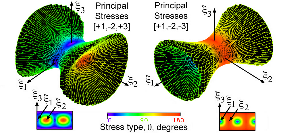
Figure 34. Stress quadric elliptical conical surface for [+1,-2,+3] and [+1,-2,-3]
These conical surfaces are interesting in that they clearly show the 3D
curved surfaces along which pure shear exists. Returning to Fig. 28 the
state of pure shear exists when σN = 0 on the plane
(P1,P2,P3) which is the same plane
shown in Fig. 30. When the stress σi is parallel to the plane
(P1,P2,P3) and perpendicular to the
unit vector, ni, the quadric surface must extend to infinity along
a collection of lines that define pure shear. This collection of lines form a
conical shape, Fig. 34. Because these cones extend to infinity these glyphs
must be truncated. After experimenting with different values for cutting off
the distance PQ in Fig. 31, the following the folowing code segment, taken
from the sq function subroutine, proved to yield acceptable results.
All tensor glyphs require a list of x, y, and z coordinates for each vertice
located on the glyph surface and a list of vertices associates with each
polygon that creates the glyph surface. The vertice list of x, y, and z
coordinates is calcuated from the distance return by the function subroutine
associate with each type of second-order tensor glyph. However the polygon
list of vertices is identically the same for all four second-order stress
tensor glyphs developed in this section. The polygon list of vertices is
generted by sequencing through the spherical coordinate angles θ and
φ defined in Fig. 33 as shown in the code segment below.
A visual summary of images (*.jpg), animations (animated *.gif), and
VRML (*.wrl) files are posted at:
At the bottom right of the visual summary web page .../Sij_results.html composite
images show the three quadric surface glyphs in Fig.s 32 and 34 together
for comparison. Off diagonal stress tensor components for these three glyphs
are zero and no rotations into a principal stress state are observed. However
the fourth glyph where σij =
(σ11, σ22, σ33,
σ12, σ13, σ23) =
(-0.069e+03, -0.018e+03, +0.274e+03, -0.074e+03, +0.021e+03, -0.041e+03) is
not in a principal stress state and a rotation into a principal stress state
is observed:
VRML-1_file /
VRML-2_file .
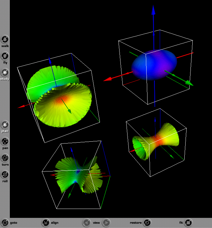
A screen capture of this VRML file comparing these four quadric surface
glyphs is shown in Fig. 35.
Figure 35. Screen capture of four second order stress tensor quadric surface
glyphs as seen using the Cortona web browser plugin.
Each glyph is labled with red, green, and blue axes which correspond to the
ξ1, ξ2, and ξ3 principal axes. Not
all VRML web browser plugins can view fonts used to label these axes. To see
the rotation of the fourth glyph a reference global axes is shown as larger
red, green, and blue axes. The global reference axes is shown to coincide
with the first quadric surface glyph, [+1,+2,+3] in the upper right corner
in Fig. 35, because the center of the first glyph coincides with the origin
of the global axes. Because the first quadric glyph is already in a principal
stress state no rotation is observed and the axes coincide. However the fourth
glyph shown in the lower left corner of Fig. 35 is observed to rotate with
respect to the global reference axes. With VRML syntax it is also not possible
to show a color legend that does not move with the global axes. Regardless of
these issues, VRML files are useful because the viewer can rotate glyphs
interactively and compare glyph shapes and orientations. If the reader does
not have a VRML plugin installed on their web browser, animations of
individual glyph rotations can be viewed using a standard web browser: select
the movie icon shown to the right of each Mercator color map. Larger clusters
of glyphs would reveal more information, however the example shown here
compares only four glyphs.
Haber Glyphs: Elliptical Disks and Rods ("keep it simple")
Haber [11] demonstrated how clusters of stress tensor glyphs in a 2D plane
could be used to study the singular stresses in the region of a crack moving
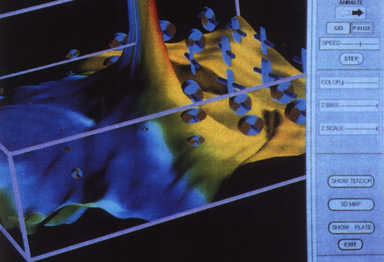
through a plate. Figure 36 shows an array of principal stress glyphs near
one of two crack tips. Here a cluster of glyphs are overlayed on top of
visual representations of two scalar properties: (1) square root of the
kinetic energy density, which is plotted along the vertical axis and seen as
a raised 2D surface plot above the cracked plate, and (2) log of the strain
energy density, which is mapped as color on the raised surface plot of kinetic
energy density. Hence the viewer can process several properties simultaneously
as the crack moves through the plate. Viewing several physical properties
simultaneously can be insightful.
Figure 36. Cluster of Stress tensor glyphs showing the gradients of second
order stress tensors uniformly distributed in the region near a moving crack
and superposed on top of scalar properties shown here as gradients, Ref. [11]:
surface height, sqrt(kinetic energy density) and color, ln(strain energy
density).
Notice that unlike the quadric surface glyphs, this glyph's shape is that of
a simple rod and an elliptical disk. Although the quadric surface reveals
additional information about the direction of the stress vector in a particular
direction, Haber's glyphs are better suited to reveal magnitudes of the
principal stress state without obscuring other properties as shown in Fig. 36.
In this case less is more when selecting a glyph type. The shape shown above,
Fig. 37, is more easily recognized when envisioning eigenvalues or principal
stresses as minor, intermediate, and major axes. Because of this simple shape
it is also easier to envision the principal directions. Perhaps glyphs can
have too much information assimulated into its shape, color, and orientation.
Although the quadric surface glyph is insightful, insight like beauty is in
the eye of the beholder. Ultimately the scientist must decide how to envision
their data. This is why the most insightful visual models are created and
customized by the scientists themselves. The same is true when constructing
the mathematical model of the physical system being studied. In both cases
insight is realized when the scientist creates both their own mathematical and
visual models.
Fig. 38. Dynamic center crack: color represents log (strain energy density),
which is mapped onto a raised surface that represents the square root of the
kinetic energy density. Notice the singularity at the crack tip, Ref. [12].
Animation: MPEG Movie (1.2Mb,141 frames)
An interference pattern observed at the center of a plate in Fig. 38 is
caused by circular stress waves emanating from the two crack tips. Here the
stress tensor glyphs have been removed to view the development of these
interference patterns in an animated movie of Fig. 38, Ref. [12]. This
animation displays the simulation - visualization results of two crack tips
growing away from the center of the plate and shows the development of this
interesting interference pattern. This stress wave interaction provided
an insightful explanation of the irregularities observed in the dynamic
crack tip stress intensity factors measured experimentally at the National
Bureau of Standards.
The numerical solution to this fracture mechanics problem provided the raw
data from which the stress tensor glyphs were created. Although these
glyphs were observed to move over large distances with the crack tip, which
is an Eulerian concept, it is interesting to note that the deformation
field is not Eulerian but Lagrangian.
Reynolds Stress Tensor Glyphs: Normal Stresses Define Shape
Moore, Schorn and Moore [13] used Reynolds stresses to study turbulent flow.
The stress tensor components are written here as a dyadic product which is
equivalent to a tensor outer product of the fluctuating velocities (u,v,w).
Once the principal directions are determined, the principal components of
the Reynolds stress tensor are found by transforming the fluctuating
velocity components,
where the repeated indices "i" implies summation and the subscript "n" on
P is not an index but implies principal directions. The dyadic product is
used again to create the components of the Reynolds stress tensor but now
in the principal stress state.
A new glyph can now be created by mapping this relationship into a cube
with the unit vector (dx,dy,dz), where sqrt(dx**2 + dy**2 + dz**2) = 1.
The mathematical development of Moore, Schorn,and Moore shown above can be
simply summarized as folows: use the normal component of stress,
σN, shown in Fig. 28, as the glyph radius. The collection
of all radii for all directions, ni, defines the glyph shape.
The use of dyadic product of velocities, uiuj to
construct the second order stress tensor is similar to taking the tensor
outer product without contracting the indices. The fact that velocity
squared with dimensions of (m/sec)2 is equivalent to the
dimensions of stress in Pascals (N/m2), is realized when
muliplying the velocity squared by density. Although common knowledge to
the community of fluid dynamicists, this dimensional analysis is noteworthy
here for those not familiar with the fact that the glyhps shown of velocity
squared are equivalent to the stress tensor by a constant scalar factor of
density.
As shown in Fig. 39 the resulting glyph is peanut shaped. Unlike the
quadric surface the largest principal stress corresponds to the largest
dimension and unlike the Haber glyph the exaggerated curvature of the
peanut shape emphasizes the anisotropy of the normal component of the
principal stress. To emphasize the shape of this glyph, Moore, Schorn
and Moore [13] mapped color contours of minimum and maximum normal
stress onto the glyph surface.
Figure 39. Comparison of the Reynolds stress tensor glyph with a quadric
surface glyph, Ref. [13].
The comparison in Fig. 39 demonstrates that the principal stress
σa along the X axis is scaled differently. For the
quadric glyph, property (i) associated with Fig. 31 requires that the
distance from the centroid to the surface equal the square root of
1/σa . For the Reynolds glyph the distance from the
centroid to the surface is simply equal to σa.
This reverses the maximum and minimum stresses mapped onto the surface.
The same is true for the other principal stresses and their directions.
The shape of the Reynolds glyph on the right in Fig. 28, is constructed
from the normal stress components, σN, of the first
order tensor, σi in all possible directions. However
the collection of all vectors envisioned normal to the surface of the
quadric glyph, on the left in Fig. 28, reveal the directions of all
possbile first order tensors, σi, necessary to maintain
equilibrium. For quadric glyphs cones reveal the collection of planes
of pure shear. Since a state of pure shear does not exist in fluids,
quadric glyphs are always seen as ellipsoids. Hence quadric glyphs
would be more useful when studying the state of pure shear in solids.
Hence each glyph envisions a different property of σi.
The choice of which glyph to use depends on what property the researcher
wants to investigate when envisioning information for insight or what
property the research wants to use when presenting information to
educate others. When envisioning information for presentation, the rule
has been not to make the graphic too "busy" or cluttered with detail to
the point of being distracting. When envisioning information for insight,
the rule is to envision as many different properties as possible in the
same space without exceeding the researcher's ability to link their
prior knowledge to the collection of graphical objects used to model
these properties. This is called the cognitive limit which depends on
the observers ability to link images to their prior scientific knowledge.
When possible, clarify by adding detail when designing a graphical model
for insight without exceeding the observer's cognitive limit. The same
could be said for presentation assuming the audience shares the same
prior scientific knowledge. Because everyones prior scientific knowledge
is different, it is important that the researcher design and create
graphical models as they anticipate the observer's prior scientific
knowledge.
Development of the Reynolds stress tensor to study turbulence in
turbomachinery was the focus of Joan and John Moore's research while
at Virginia Tech. Their research continues with recent advances on how
Reynolds stress tensor glyphs are used to study turbulence. On the
Moores' web pages are
links to their new text book, "Functional Reynolds Stress Modeling". This
research is an excellent example of how graphic models are developed
within the context the science as understood by the researcher. Because
of this context these customized graphic models become insightful by
those who understand the science. Because of this context, results of
these graphical models can also be used for presentation within the
scientific community.
When envisioning information for insight, more information is obtained
when arranging these glyphs in an evenly spaced array, compared to a
conventional use of contour lines and vectors. To clarify add detail.
These two formats are compared in Fig. 40 which is a composite of Fig.s
2 and Fig. 8 taken from Ref. [13]. In the lower left region of Fig. 40
the glyph size is scaled to represent the magnitude of the prinicipal
stresses. The larger glyphs represent larger stresses which can obscure
or hide information on adjacent glyphs.
Figure 40. Comparison of Reynolds stress tensor glyphs with contour
lines, Fig. 2 (left) and Fig. 8 (right) taken from Ref. [13]. A
larger format of this figure is made
available here and in Ref. [13].
The Reynolds and quadric glyphs are compared again in Fig. 41, by using
different color mapping proposed in Fig.s 28 and 31. The color contours
mapped onto the surface in Fig.s 39 and 40 are scaled with respect to
the minimum and maximum normal stresses which can be very useful for
both insight and presentation. However if the researcher wants to
envision the direction of the orientation of the first order stress
tensor, σi, that reveals the orientation of the pure
shear stress state, this choice is better shown in Fig. 41 using the
quadric glyph. Again the point is made that envisioning information
should be a choice within the intent to provide scientific insight or
to educate others, e.g. "presentation", who share the researcher's
prior scientific knowledge.
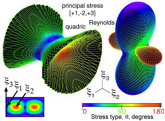
Figure 41. Comparison of Reynolds and quadric glyphs using a color
gradient on the surface that shows stress type, defined in Fig. 28,
for a principal stress state of [+1,-2,+3].
By mapping stress type as color, the green shear stress is observed to
coincide with the conical surface of the quadric glyph, where shear is
expected, but shear is observed on the Reynolds glyph surface where it
was not expected. This new information reveals that although the shape
of the Reynolds glyph is defined only by using the normal stress
components, σN, shear stress can be envision as well.
The distance from the centroid of the Reynolds glyph to the surface is
calculated using the function subroutine, sn, shown below.
A comparision similar to that done for different types of principal
stress states in Fig. 35 is shown here for Reynolds glyphs in Fig. 42.
Again the
VRML-1
and
VRML-2
files can be download into a web plugin
viewer or *.gif animated rotations of the same Reynolds glyphs can be
viewed from movie icon links on the
Sij_results.html
web page.
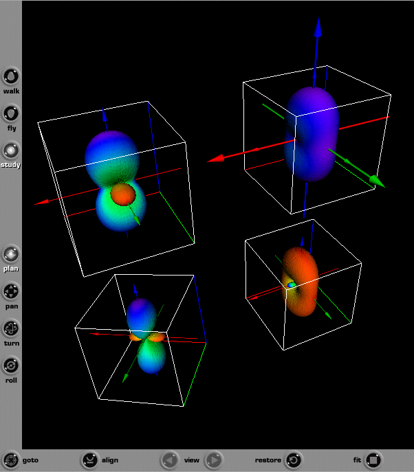
Figure 42. Screen capture of four second order stress tensor Reynolds
glyphs as seen using the Cortona web browser plugin. Web links are
provided for
VRML-1
and
VRML-2
files.
HWY Glyphs: Shear Stresses Define Shape
The HWY stress glyph is named in honor of it's authors, Hashash,
Wotring, and Yao [14], who emphasized envisioning the shear component,
σS, of the first order stress tensor,
σi shown in Fig. 28. The HWY glyph was developed for
a geotechnical application where the shear component of the first
order stress tensor was of interest. The quadric, Reynolds, and HWY
glyphs are compared in Fig. 43 using the color mapping proposed in
Fig.s 28 and 31.
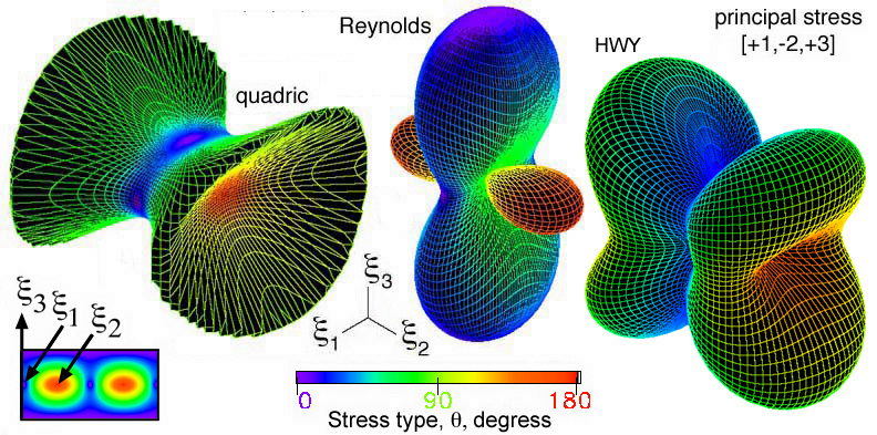
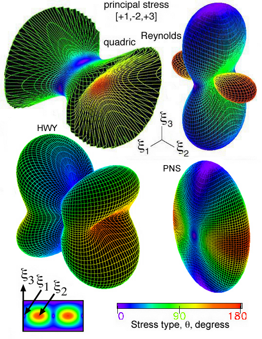
Figure 43. Comparison of quadric, Reynolds and HWY glyphs using a color
gradient on the surface that shows stress type for a principal stress
state of [+1,-2,+3].
The distance from the centroid of the HWY glyph to the surface is the
shear component, σS, of the first order stress,
σi, shown in Fig. 28. This shear component,
σS, is calculated using the function
subroutine, ss, shown below.
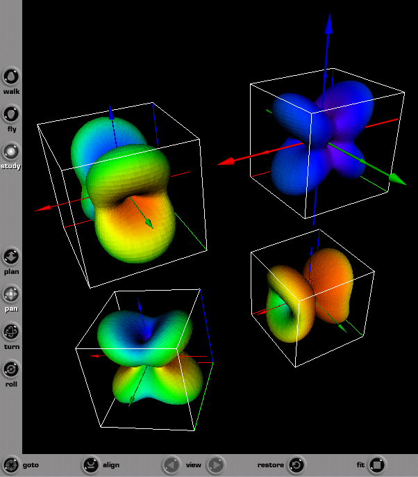
Figure 44. Screen capture of four second order stress tensor HWY glyphs
as seen using the Cortona web browser plugin. Web links are provided for
VRML-1
and
VRML-2
files.
PNS glyph: Principal Normal Stresses Define Ellipsoidal Shape
Unlike the Quadric, Reynolds, and HWY glyphs, the PNS glyph is always an
ellipsoid whose major, intermediate, and major axes corresponds to the
Principal Normal Stresses (PNS)
(σa,σb,σc). The PNS glyph
was developed by M. Yaman and R.D. Kriz where the intent was to keep the
glyph shape simple like the Haber glyph, but unlike the Haber glyph provide
additional informaton of the stress type as color mapped onto the PNS glyph
surface. The quadric, Reynolds, HWY, and PNS glyphs are compared in Fig. 45
using the color mapping proposed in Fig.s 28 and 31.
Figure 45. Comparison of quadric, Reynolds, HWY, and PNS glyphs using a
color gradient on the surface that shows stress type for a principal
stress state of [+1,-2,+3].
The distance from the centroid of the PNS glyph to the surface of and
ellipsoid whose major, intermediate, and minor axis are defined by the
principal stresses (σa,σb,σc).
This distance is returned as a radius, e, and calculated using the
function subroutine, e, shown below.
A comparison similar to that done for different types of principal stress
states in Fig.s 35, 42, and 44 is shown here for PNS glyphs in Fig. 46.
Again the
VRML-1
and
VRML-2
files can be download into a web plugin viewer
or *.gif animated rotations of the same PNS glyphs can be viewed from movie
icon links on the
Sij_results.html
web page.
Figure 46. Screen capture of four second order stress tensor PNS glyphs
as seen using the Cortona web browser plugin. Web links are provided for
VRML-1
and
VRML-2 files.
A visual summary of these four glyphs were used to study two different types
of residual stresses gradients: 1) residual stresses near welds, and 2) surface
residual stresses induced by plastic deformations (shot peening) in a Titanium
alloy (Ti-6Al-4V). This research was collaboration with Professor M. Harting, and
Mr. Mecit Yaman, Ph.D candidate, in the Department of Physics at the University
of Cape Town, South Africa and Dr. Ron Kriz, Department of Engineering Science
and Mechanics, Virginia Tech, Blacksburg, Viriginia, USA. A complete description
of results from this collaboration is available by going to the web link:
Residual Stress Gradient Visualization. However a brief summary is include
here as an example of how an array of second-order stress tensor glyphs can be
used to study residual stresses in welds and stress gradients near surfaces due
to plastic deformation.
The first four images show the quadric, Reynolds, HWY, and PNS glyphs superposed
on top of the weld structure, Fig. 47. Only the principal stresses are shown in
Fig. 47, which does not show the rotations into the principal stress state.
Images in Fig. 47 are scaled to fit the width of a typical web page. To view
these images in more detail, a
web link of results in a larger image format
is provided here for reference. For comparison only the quadric glyph type for
"as-welded" and "post-heat-treated" are shown in one file where the rotations
of the various principal stress states can be compared using the VRML file
format, Fig. 48.
Figure 47. Quadric, Reynolds, HWY, and PNS glyphs for the "as-welded"
condition is superposed onto weld structure. The "post-heat-treated"
condition not shown
A
web link of all results including large image formats is provided here
for reference.
Figure 48. Quadric glyph arrays of "as-welded" and "post-heat-treated" combined
into single
VRML-1 and
VRML-2 file format where principal directions are shown as rotated glyphs.
This collection of second-order stress tensor glyphs when organized into an
array and superposed on top of the weld structures can facilitate the analysis
of how changes in residual stresses correspond to weld structure. In Fig. 48
results in the "as-welded" conditions are observed to change when compared
with the "post-heat-treated" condition. This large array of glyphs shown
in Fig. 48 would benefit from an immersive virtual environment, where the
viewer can move through space and view these stress tensor gradients
immersively by using three-dimensional head tracking. This is possible by
renaming the VRML-1 file extension from *.wrl to the Inventor format *.iv.
This is possible because when SGI was the leader in graphical interface,
the VRML-1 and Inventor file formats were interchangeable. Since most
immersive application programming interfaces (APIs) can load Inventor files,
the VRML-1 files can be viewed interactively both at the desktop computer
using a Web browser plugin and in an immersive environment. Immersive
environments are particulary useful when interpreting large arrays of data
in a three-dimensional gradient format.
Briefly, results of stress gradients are also shown near a surface induced by
plastic deformation (shot peening) in a Titanium alloy. Again web links to
VRML file formats are provided for downloading into Web browser plugins
or into immersive environments. Results are shown as glyph-gradients near
the surface where Quadric, Reynolds, HWY, and PNS glyphs are shown together
for comparison.
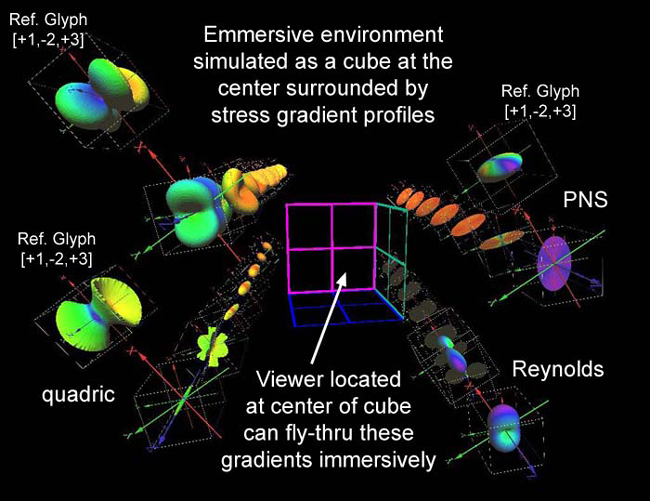
Figure 50. Residual stress profiles loaded into an immersive environment where
the cube shown at the center visually simulates the location of the 10' by 10'
by 10' walls where stereo images are projected.
These results show a significant change in the principal stresses near the
surface, but only a slight rotational gradient with depth in both Fig.s 49
and 50. Immersive environments proved to be useful when large arrays of glyphs
were created.
Stress Tensor Gradients in One Dimension: Tensor Tubes
Many problems in continuum mechanics emphasize continuous changes in tensor properties:
such as the comoving derivative of a property associated with a fluid particle moving
through a fluid in Eulerian space or continuous lines of principal stress in a solid
where the deformation field is defined in Lagrangian space. In the Haber glyph example
clusters of stress tensors were used to envision a stress gradient near a crack tip
in Lagragian space. However when this same array of stress glyphs moved with the crack
tip, these stress gradients were envisioned to change as they moved through space,
which is an Eulerian concept. This regularly space array of Haber glyphs shown in
Fig. 36 must be spaced so as not to obscure the isosurfaces of kinetic energy density
and color gradients of strain energy density. Unfortunately there is a large stress
gradient near crack tips, which requires closer spacing of stress tensor glyphs to
accurately recover the gradient in this region. These are conflicting issues that can
be resovled by creating continuous stress tensor tubes.
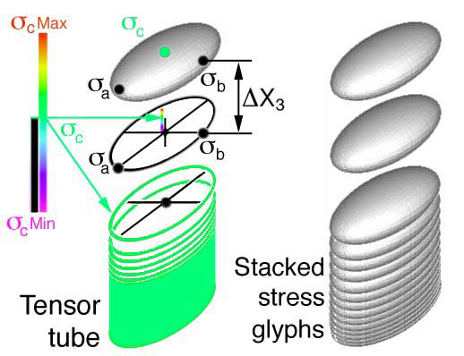
Delmarcelle, Hesselink and Helman [15, 16] envisioned continuous changes of second
order tensor fields as a stress tensor tube. Stress tensor tubes are an extension of
the Haber glyph, where the perimeter of the Haber glyph
(σb,σc) is used to create the tube's
surface and the length of the rod (σa) is mapped as color onto the
perimeter. This technique is used to envision very small changes in the second order
stress tensor corresponding to small changes in distance, ΔX3. The
components (σa,σb,σc) used to
construct the tube can also be envisioned as the major, intermediate, and minor axes
of the PNS stress tensor ellipsoid, Fig. 51. Here the minor axes, σc
is used to map color on the perimeter.
Figure 51. Creation of stress tensor tubes from stacked PNS ellipsoidal glyphs.
In Fig. 52 the center of the two glyph tubes propagate upward along trajectories or
line s that represent the direction (eigenvector) of the largest compressive stress.
In this figure the color represents the magnitude of the largest compressive stress
(the minor eigenvalue). The shape of the tube represents the magnitudes of the other
two eigenvalues. Similar trajectories near the bottom of the figure for the other
two eigenvectors take a shape that is everywhere perpendicular to the most
compressive stress. These flat tened tubes show that one of the eigenvalues must be
close to zero.
Figure 52. Elastic-stress tensor field in a solid induced by two compressive forces
applied at the top surface, Refs. [15, 16].
The next figure, Fig. 53, shows how the shape of the tubes in Fig. 52 change if an
additional tension force is applied at the top surface (the exact location is not
specified) Ref. [15, 16]. The shape of these glyphs are shown to change with
increasing tension force (a) -> (b) -> (c) -> (d).
Figure 53. Elastic-stress tensor field glyphs shape changed by additional tension
surface force. Glyph (c) shows that one of the principal stresses is zero,
Refs. [15, 16]
In this example the magnitude of the compressive principal stress was mapped as
color on the continuous stress tensor glyph. Many other combinations are discussed
in Ref. [15,16].
Tensor tubes prove to be useful when envisioning gradients in one direction: e.g.
in Fig. 51 as ΔX3 approaches zero the stacked PNS elllipsoidal
glyphs obscure informaton in the X3 direction, however color can be used
to recover this information but only in X3 direction. Since mathematical
concept of gradients is three-dimensional, another visual approach is explored
that envisions gradients of stress tensors in all three-dimensions.
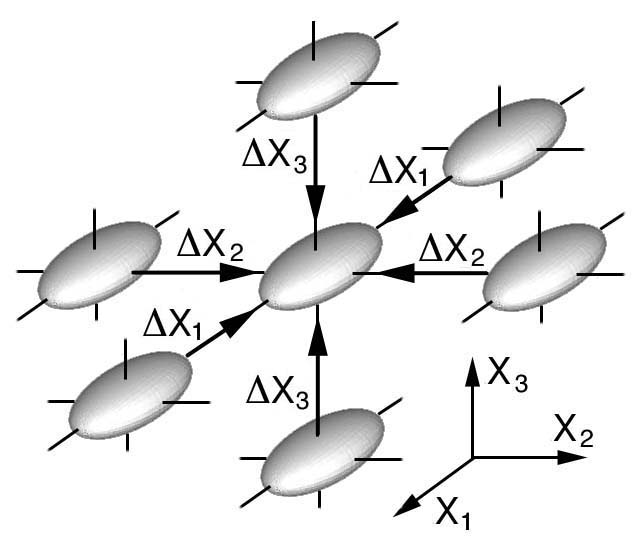
Point Stress Tensor Gradients in Three Dimensions
Gradients of second order stress tensors in three-dimensions can be envisioned by
drawing a collection of evenly space stress tensor glyphs in RCC space. Either
quadric, Haber, HWY, or PNS glyphs can be used, however in Fig. 54 the PNS
ellipsoidal glyph is used for simplicity. The center PNS glyph is used as the
reference glyph and the surrounding PNS glyphs are located at evenly spaced distances,
ΔX1, ΔX2, and ΔX3, which would be
seen as a collection of glyphs located to the north, south, east, west, front, and
back of the center glyph, Fig. 54.
Figure 54. Stress glyph gradient where there is no change in shape or orientation
of the nearest neighboring stress glyphs collapsing onto the center glyph.
If the glyph spacing is small but the 3D collection of glyphs does not obscure
the viewer from seeing how glyphs change their shape and orientation as these
glyphs collapse onto the center glyph, than the viewer is seeing a stress
gradient within a discrete change in space.
In the limit as ΔXk goes to zero, Eqn. (32) reduces to
which transforms as a third order tensor. Summing forces requires a contraction
on the "i" and "k" indices which yields,
The collection of glyphs in Fig. 54 envisions the gradient collapsing or
expanding on the center glyph but only for one particular orientation,
σji,j=0, which satisfies equilibrium in this particular
direction. However equilibrium is a law, therefore it must exist in all
possible directions and arbitrarily so.
This idea of invariance in a physical sense is the same as invariance
in a mathematical sense by transforming each term in the equlibrium
equation, σ'kj,k=0. The apostrophy
symbolically represents this arbitrary mathematical transformation.
The fact that the equation maintains it's form after such an arbitrary
transformation is the idea of mathematical invariance.
How would we envision a collection of glyphs that would visually represent
a gradient in any arbitrary direction? What would this 3D image look like?
One possible implementation of this idea is to envision an infinite set of
stress quadric surface glyphs propagating outward from the center glyph in
all possible directions simultaneously. This collection of stress tensor
glyphs would be expanding not collapsing. This idea is similar to Huygen's
principle for 2D plane waves eminating from a point, but using 3D stress
quadric surface glyphs instead. An expanding 3D small multiple of 3D objects.
This image would be difficult to envision and represents a limit in our
visual cognitive ability to envision stress gradients in any arbitrary
direction. Although difficult for mortals to envision, such a surface
would be seen as symmetric -- a necessary requirement to satisfy
equilibrium and it's gradients.
Glyphs can also be used to better understand higher order tensors. For example,
fourth order stiffness tensor, Cijkl, can also be envisioned using
simple glyphs. The fourth order stiffness tensor relates all of the components of
the second-order strain tensor, lkl to the second-order stress tensor,
σij.
If the indices are expanded, Eqn. (36) reduces to eigen-value problem, where the
eigenvalues, ρv2, are related to the wave speeds, v, and density,
ρ, and the eigenvectors are the particle vibration directions, pk,
of Eqn. (36). The surface shown in Fig. 55 is generated by prescribing all
possible directions, νi and νj in Eqn. (36) and
mapping out all of these solutions as a glyph: the eigen-value solutions, wave
velocities, v, is the distance from the geomtric center to the surface and
the eigen-vector solutions are used to map a color for each eigen-value solution
at the point where the pointing vector, νi, intersects the surface.
Since both the eigen-values and their corresponding eigen-vectors are functions
only of Cijkl, see Eqn. (36), then the surface shape and colors shown
in Fig. 55 can be used to envision this fourth-order stiffness tensor. Because
all terms of the fourth-order tensor were used to calculate the wave surface and
its colors we see the relationship between the eigenvalues and their
corresponding eigenvectors at every point on this surface. We can also observe
the spin properties of the displacement fields as color gradients that exist
near degeneracies in the eigen-values that appear as the concave portion of the
wave surface that collapse to a point (see black region). It is through these
degeneracies that wave surfaces can interconnect into single continuous
connected wave surfaces (mode-transitions at eigen-value
degeneracies ) Kriz and Ledbetter [18]. At these same degeneracies internal
conical refraction exist. Again the mathematical invariant property of tensor
equations is used here to develop an understanding of the physical properties
envisioned in Fig. 55.
Figure 55. Fourth order stiffness tensor glyph for a single crystal of Calcium
Formate (orthorhombic symmetry). Shape of surface maps the wave velocity for
the fastest of the two quasi-transverse waves [17,18]. Here only the intermediate
wave surface is shown. The outermost and inner most wave surfaces are not shown.
Visual Numerics PV-Wave software, Ref. [21], maps the particle vibration directions
onto the glyph surface as color: black corresponds to longitudinal (0o)
vibration directions and white corresponds to transverse (90o). A mode
transitions are highlighted as red.
Several researchers [17, 18, 19, 20] have used Christoffel's equation to study the
symmetries of waves propagating in different crystal class symmetries. A summary
of results for differnt crystal class symmetries is present here as an example.
Envisioning 3D Wavesurfaces as Cijkl-glyphs:
The reader interested in the tensor approach to this dynamic problem is encouraged
to study references [17, 18, 19]. For the reader only interested in the previous
example of the principal stress state, it is not difficult to show that equation
(36) reduces to equation (15). This is a simple task using tensor notation. Both
equations are rewritten here to facilite the comparison.
Eqn. (36) reduces to the same tensor equation that defines the eigen-value
problem, Eqn. (15),
Except for the term, βij which is contracted with the fourth order
stiffness tensor, Cijkl, see Eqn. (37), the βij term in
Eqn. (40) is not just a simple second order tensor like σij, but
derives its properties from a higher order tensor and hence enjoys a much richer
surface topology shown in Fig. 55 then the simple PNS ellipsoid geometry for
σij.
The fact that Eqn.s (36) and (15) have the same invariant tensoral form supports
the idea, proposed in section Point Stress Tensor Gradients in Three
Dimensions, that a continuous stress gradient in all directions, envisioned
as a surface generated by an infinite set of stress quadric surfaces expanding
out from the center glyph, would generate a surface similar to an infinite set
of 2D plane waves eminating from a point. Indeed the surface generated by Eqn.
(36), Fig. 56, starts at a point, which is envisioned as a spherical dilatation
constructed of an infinite number of 2D plane waves expanding out in all
directions simultaneously. Each of these plane waves travels in a specific
direction called the pointing vector, νi, at a speed that
corresponds to elastic properties in the same direction. Hence, plane waves
traveling in different directions in an anisotropic material will travel at
different speeds and the continuous collection of all connected plane waves,
although initially a sphere, soon deviates into a non-spherical shape simply
because a plane wave will travel faster in stiffer directions and slower in
less stiff directions. The final result is envisioned as three wave surfaces
connected together through their points of degeneracies as shown in Fig. 56
and also in the schematic in the upper left corner of Fig. 55.
Figure 56. Complete solution to Christoffel's Eqn. (36) for Calcium Formate
envisioned using translucency:
VRML-1 and
VRML-2.
In Fig. 56 the outer two, faster, wave surfaces are shown using translucency so
that the inner two, slower, wave surface structures can be seen as a single
surface connected to the outer surface. The single connected surface is seen
schematically in the upper left corner of Fig. 55 and immersively by using head
tracking in a back projected immersive environment. Together these three
surfaces are the collection of all eigen-values solutions mapped out in all
directions. This is similar to mapping out all solutions to Cauchy's equation,
which is equivalent to the statement of equilibrium when mapping out the stress
quadric surface, Eqn. (27). Hence the mathematical invariance of Cauchy's
equation envisions static equilibrium in Fig.s 32 and 34, the same as
invariance of Christoffel's equation is used to envision dynamic equilibrium
in Fig. 56. This supports the idea proposed in the introduction, that
"enhanced understanding is realized when graphical models are created
together with the development of the mathematical models". Because Eqn.s (36)
and (15) are tensor equations, information embedded in Fig.s 32, 34, and 56
facilitates discovery and insight that transcends presentational value.
These 3D wave surfaces propagate through anisotropic materials modelled at the
macroscale as a continuum. However it is well known that anisotropy is a
property associated with different crystal class symmetries modelled as unit
cells at the nanoscale. These continuum and nanoscale models can be combined
and compared visually by embedding a continuum of unit cells inside connected
translucent 3D wavesurfaces. This visual comparison is insightful in the sense
that the wave surface bulges correspond to the orientations of the unit cell
bonds, Ref.[22]. This idea was also submitted to the 2003 NSF Science and
Engineering Visualization Challenge,
Visualization of Structure-Property Relationships:
Spanning the Length Scales (nano to macro) Ref.[23]. Linking the macro
(continuum) and nanoscales visually is shown in Fig. 57. Insight is NOT realized
by well designed graphics, but rather by prior knowledge and a fundamental
understanding of tensors, tensor equations, continuum mechanics, unit cell crystal
class symmetries. Well designed graphics is necessary but realizing a cognitive
link to a fundamental understanding of the science is the sufficient condition
for insight. Unfortunately insight within a scientific context was not a criterion
used by the National Science Foundation in their contest.
Future Cijkl-glyphs will include a continuum of unit cells corresponding
to their crystal class symmetries and principal material axes used to define glyph
orientation.
Following the same idea presented in the development of Eqn. (40), it is possible
to show that the Cijkl term in Eqn. (36) is a contraction of a higher
order tensor, that is the sixth order tensor, Cijklmn, associated with
stress induced anisotropy, Ref.[24].
This is on going research which will be posted as results become available.
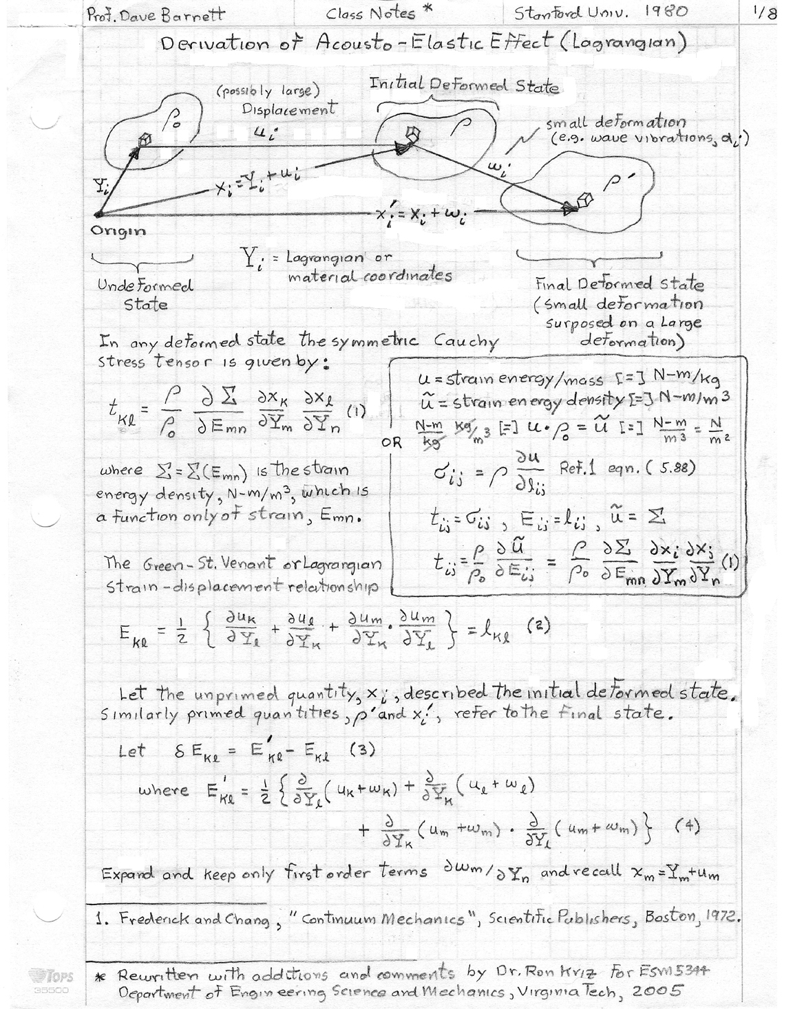
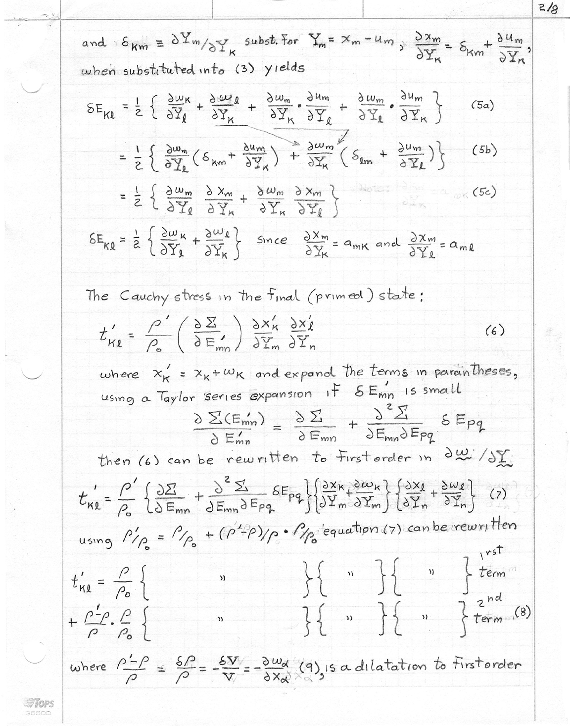
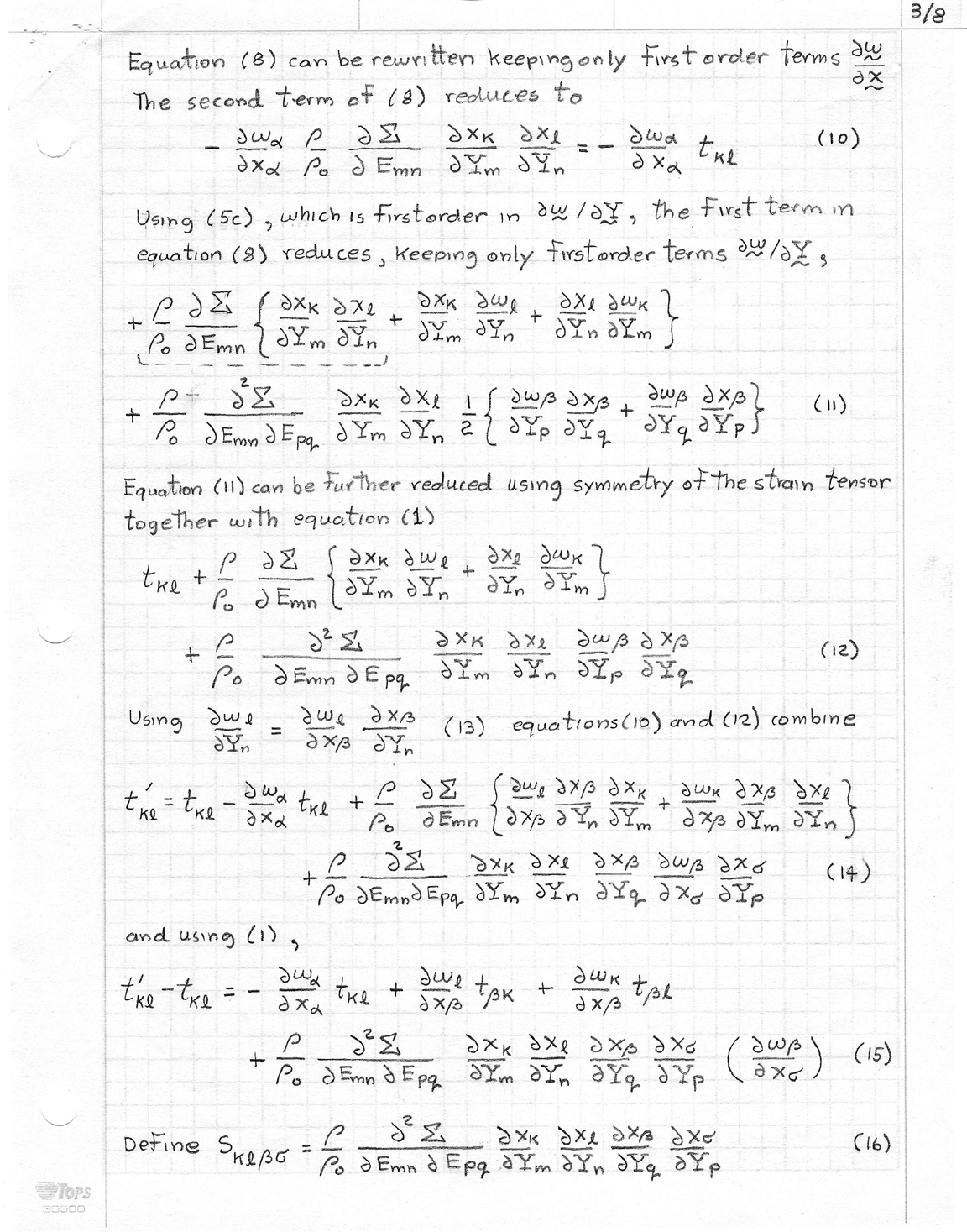
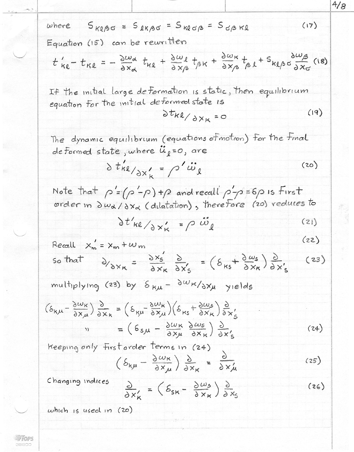
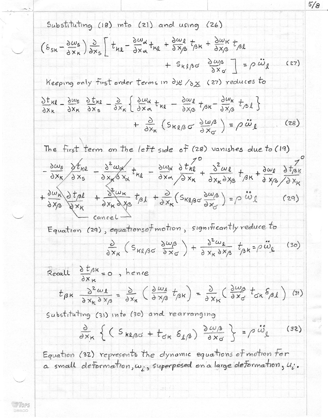
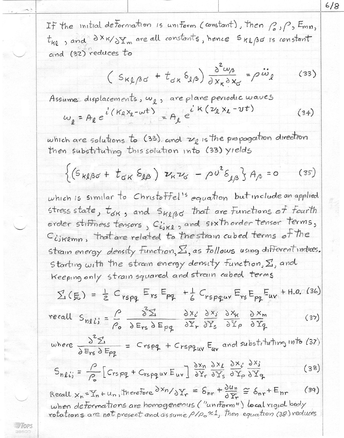
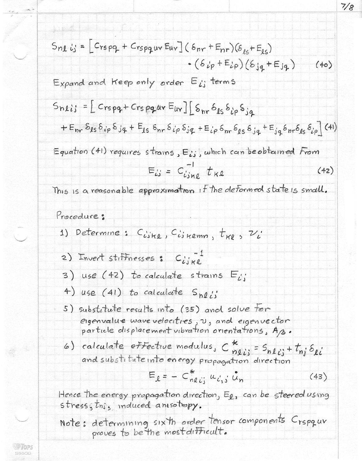
Notes on the derivation of acousto-elastic effect are provided that show how
equation (36) can be modified to include an effective fourth order tensor that
is a function of an applied stress and the sixth order tensor Cijklmn,
see equation (35) in the derivation:
Page-1,
Page-2,
Page-3,
Page-4,
Page-5,
Page-6,
Page-7,
Page-8,
Page-9,
Page-10,
Page-11,
Page-12,
Page-13,
Page-14,
Page-15,
Page-16,
Page-17,
Page-18,
Page-19,
Current: http://www.esm.rkriz.net/classes/ESM5344/ESM5344_NoteBook/ESM4714/methods/EEG.htmlEnvisioning Second-Order Stress Tensors, σij
σ'ij = air ajs σrs (10)
X'i = aij Xj (11)
σi = σji nj (12)
σi = σ ni, where σ = σN (13)
σi = σji nj = σ δij nj        (14)

( σji - σ δij ) nj= 0         (15)
 (16)
(16)
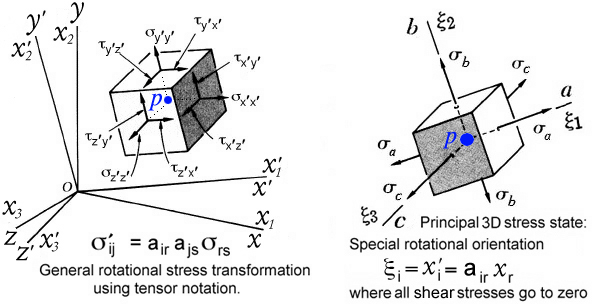
Figure 29. Rotation of differential element into the principal stress state.
c
c read and write s(i,j) matrix as a symmetric second order tensor
     read(5,101)s(1,1),s(2,2),s(3,3),s(1,2),s(1,3),s(2,3)
    *,x(im),y(im),z(im)
     s(2,1)=s(1,2)
     s(3,1)=s(1,3)
     s(3,2)=s(2,3)
     write(6,200) n,itmax,eps1,eps2,eps3
     do 2 i=1,n
   2 write(6,201) (s(i,j),j=1,n)
c
c Save original s(i,j) matrix as ss(i,j) for later calcuations
c because s(i,j) is modified by subroutine jacobi.
     do 3 i=1,n
     do 3 j=1,n
   3 ss(i,j)=s(i,j)
c
c  compute eigenvalues and eigenvectors
      call jacobi(n,s,eval,evect,itmax,eps1,eps2,eps3)
Given the nine components, n=3 (3 rows and columns), of the stress tensor,
s(i,j), subroutine jacobi returns a total of three eigen-values and a
corresponding set of three eigen-vectors. For each i-th eigen-value, eval(i),
there is a corresponding eigen-vector, evect(i,j), with three components,
j=1,2,3. These eigen-vector components correspond to the direction cosines,
ξj, in Eqn (16) which defines the orientation of the plane
(P1,P2,P3) in Fig. 28, when
σS = 0. Since there are three eigen-values there is a set of
three eigen-vectors, evect(i,j), that define the directions of the three
principal planes shown in Fig. 29. Together this collection of direction
cosines is related to the rotational transformaton matrix, aij,
used in Eqn.s (10) and (11), however subroutine jacobi stores eigen-vectors
column-wise (j-th eigen-values) for printing. Hence the eigen-vector matrix
created by subroutine jacobi must be transposed before being set equal to the
transformation matrix, aij. From this transformation matrix Euler
angles are calculated.
c
c Subroutine jacobi stores eigenvectors column-wise for printing
c which is transposed to row-wise convention if eigenvectors are
c to be equated to the tensor transformation matrix a(i,j). This
c transposition is confirmed to be correct by the second order
c tensor transformation of the stress tensor into the principal
c stress state: sp(i,j)=a(i,k)*a(j,m)*ss(k,m). NOTE:
c transposition effects the Euler angle calculations
     do 4 i=1,n
     do 4 j=1,n
   4 a(i,j)=evect(j,i)
Euler angles are the preferred method of rotating three-dimensional objects
in many graphic programs. Below we develop a general method for extracting
Euler angles from a tranformation matrix, aij.
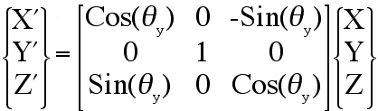 (17),
(17),
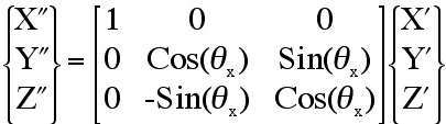 (18),
(18),
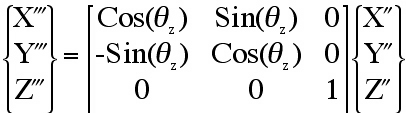 (19).
(19). (20),
(20),
 (21)
(21)
 (22)
(22)
 (23)
(23)
 (24)
(24)
c
c calculate angles from unprimed (reference) to primed (rotated) axes
c using the transformation matrix a(i,j) = transpose of evect(i,j)
     angx=acos(a(1,1))*180.0/pi
     angy=acos(a(2,2))*180.0/pi
     angz=acos(a(3,3))*180.0/pi
c
c calculate Euler angles (degrees)
     aa=-a(3,2)
     bb=+a(3,1)/a(3,3)
     cc=+a(1,2)/a(2,2)
     eulerangx=asin(aa)*180.0/pi
     eulerangy=atan(bb)*180.0/pi
     eulerangz=atan(cc)*180.0/pi
| σij - σ δij | = 0          (25)

    (26)
(26)
F(ξi) = σij ξi ξj = k2 (27)
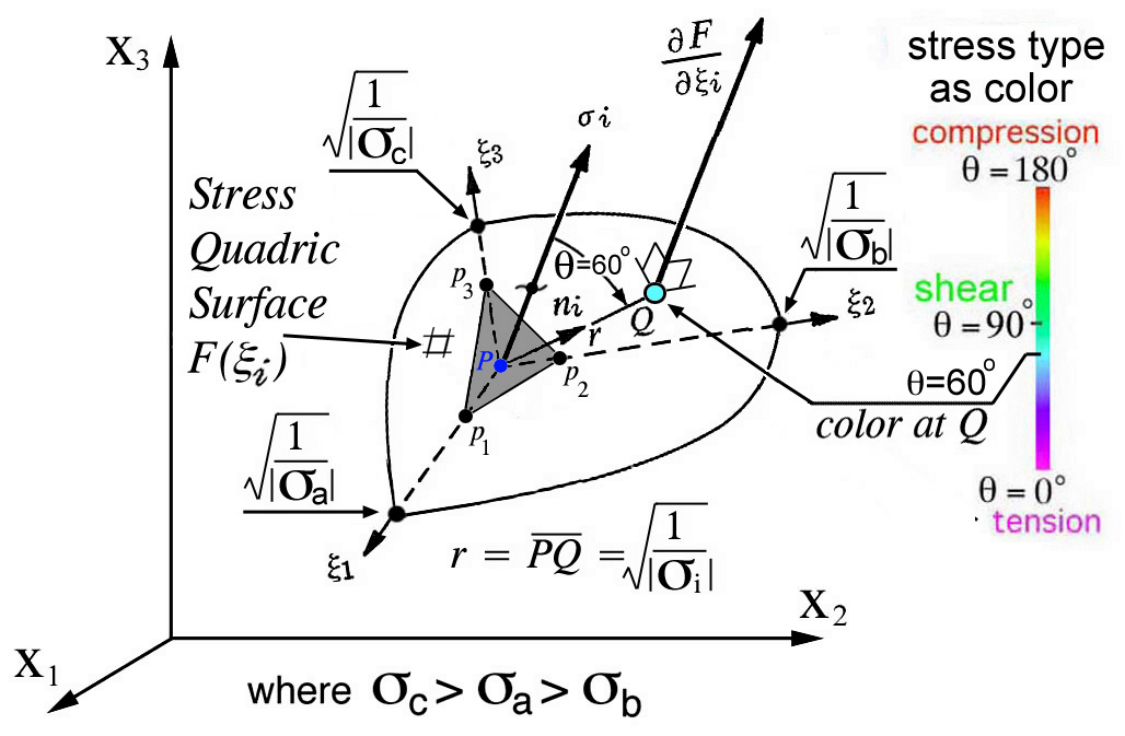
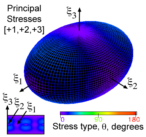
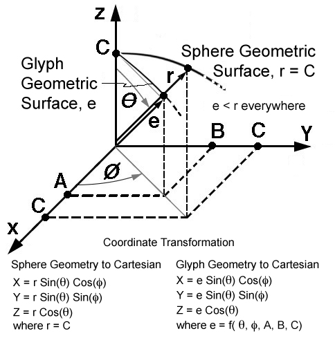
Figure 33. Spherical coordinate system used to generate glyph topology.
      function sq(p,t,s11,s12,s13,s22,s23,s33)
c
c***********************************************************************
c* Calculate distance, "sq", from the quadric surface to the geometric *
c* glyph centroid which is equivalent to the inverse of the square     *
c* root of the normal stress of the first order stress tensor, Si,     *
c* which acts in equilibrium with the second order stress tensor, Sij, *
c* definded by Cauchy's relations.  In the direction defined by        *
c* spherical coordinates: (theta,phi)                                  *
c* where  theta = t  0->180 degress along the longitude                *
c*        phi = p    0->360 degrees along the latitute                 *
c***********************************************************************
c
c   Define unit vector direction cosines
      d1=sin(t)*cos(p)
      d2=sin(t)*sin(p)
      d3=cos(t)
c
c  Calculate components of the first order stress tensor from the
c  second order stress tensor terms using Cauchy's relationship
      s1=s11*d1+s12*d2+s13*d3
      s2=s12*d1+s22*d2+s23*d3
      s3=s13*d1+s23*d2+s33*d3
c
c  Calculate the normal, "sn", component of the first order stress tensor
c  projected in the direction of the unit normal perpendicular to the
c  plane on which the first order stress tensor is acting.
      sn=s1*d1+s2*d2+s3*d3
c
c  Calcualte quadric surface distance, sq
      trace=(1./abs(s11)+1./abs(s22)+1./abs(s33))/3.0
      sq=sqrt(trace/abs(sn))
c     write(6,12)sn,sq
      if(sq.gt.3.2*trace)sq=3.2*trace
c  12 format(' *********************************************************
c    ************************',/,' sn=',e12.5,' sq=',e12.5)
c
      return
      end
When all of the principal stresses are positive the quadric surface is an
ellipsoid, Fig. 32. When one or two of the principal stresses are negative
the quadric surface is a symmetric three dimensional elliptic cone, Fig. 34.
Because color gradients of stress type are distorted when mapped onto the
irregular shapes of the conical quadric surfaces, Mercator maps of the
stress type color gradient are seen undistorted below each image.
      trace=(1./abs(s11)+1./abs(s22)+1./abs(s33))/3.0
      sq=sqrt(trace/abs(sn))
      if(sq.gt.3.2*trace)sq=3.2*trace
As expected the green color near pure shear is seen on the truncated portion
of the glyphs shown in Fig. 34. Unfortunately the green color corresponding to
pure shear at infinity has been truncated.
      program m_glyph_poly_tp
c
c***********************************************************************
c program m_glyph_poly_tp generates polygon file or "connectivity" data*
c file assigning polygon numbers to vertice numbers. Together with each*
c of the vertice data files associated with PNS, HWY, Reynolds, and the*
c quadric glyph, this polygon data file defines each of the four Sij   *
c second order stress tensor 3D glyph geometries.                      *
c***********************************************************************
c
      open(6,file='tp_poly.out',status='unknown',err=8888)
      open(8,file='d_poly.dat',status='unknown',err=8888)
      pi=acos(-1.)
c
c  360 and 180 Resolution Divided by 3
      nphi=121
      rphi=360.0
      ntheta=61
      rtheta=180.0
c
c calcuate the total number of vertices
      ivert=0
      do 200 iphi=1,nphi
      do 100 itheta=1,ntheta
      ivert=ivert+1
  100 continue
  200 continue
      write(6,210)ivert
  210 format(' Total number of vertices=',i7)
c
c   create polygonal portion of the wave surface topology
      ipnt1=0
      iarray=0
      nphm1=nphi-1
      nthm1=ntheta-1
      do 400 iphi=1,nphm1
      do 300 itheta=1,nthm1
      theta=(itheta-1)*rtheta/(nthm1-1)
      ipnt2=ipnt1+1
      ipnt4=ipnt1+ntheta
      ipnt3=ipnt4+1
      if (theta.eq.0.0)then
      n=3
      write(8,255)n,ipnt1,ipnt2,ipnt3
  255 format(4(1x,i5))
      elseif (theta.eq.180.0)then
      n=3
      write(8,255)n,ipnt1,ipnt2,ipnt4
      else
      n=4
      write(8,260)n,ipnt1,ipnt2,ipnt3,ipnt4
  260 format(5(1x,i5))
      endif
      iarray=iarray+n+1
      ipnt1=ipnt1+1
      ielmnt=ielmnt+1
  300 continue
      ipnt1=ipnt1+1
  400 continue
      write(6,500)iarray
  500 format(' Total number of polygons=',i7)
c
 8888 stop
      end
A complete summary of these examples with the code that was used to generate
images of stress quadric glyphs and other glyph types are posted at:
 (28)
(28)
 (29)
(29)
 (30)
(30)
 (31)
(31)
      function sn(p,t,s11,s12,s13,s22,s23,s33)
c
c***********************************************************************
c* Calculate normal component, "sn" of the first order stress tensor   *
c* acting in the direction of the unit vector normal to the plane on   *
c* which the first order stress tensor, Si, acts in equilibrium with   *
c* the second order stress tensor, Sij, defined by Cauchy's relation.  *
c* In the direction defined by spherical coordinates: (theta,phi)      *
c* where  theta = t  0->180 degress along the longitude                *
c*        phi = p    0->360 degrees along the latitute                 *
c***********************************************************************
c
c   Define unit vector direction cosines
      d1=sin(t)*cos(p)
      d2=sin(t)*sin(p)
      d3=cos(t)
c
c  Calculate components of the first order stress tensor from the
c  second order stress tensor terms` using Cauchy's relationship
      s1=s11*d1+s12*d2+s13*d3
      s2=s12*d1+s22*d2+s23*d3
      s3=s13*d1+s23*d2+s33*d3
c
c  Calculate the normal component, "sn" of first order stress tensor
c  projected in the direction of the unit normal perpendicular to the
c  plane on which the first order stress tensor is acting.
      sn=s1*d1+s2*d2+s3*d3
c
      return
      end
      function ss(p,t,s11,s12,s13,s22,s23,s33)
c
c***********************************************************************
c* Calculate shear component, "ss", of the first order stress tensor   *
c* acting in the direction of the unit vector normal to the plane on   *
c* which the first order stress tensor, Si, acts in equilibrium with   *
c* the second order stress tensor, Sij, defined by Cauchy's relation.  *
c* In the direction defined by spherical coordinates: (theta,phi)      *
c* where  theta = t  0->180 degress along the longitude                *
c*        phi = p    0->360 degrees along the latitute                 *
c***********************************************************************
c
c   Define unit vector direction cosines
      d1=sin(t)*cos(p)
      d2=sin(t)*sin(p)
      d3=cos(t)
c
c  Calculate components of the first order stress tensor from the
c  second order stress tensor terms using Cauchy's relationship
      s1=s11*d1+s12*d2+s13*d3
      s2=s12*d1+s22*d2+s23*d3
      s3=s13*d1+s23*d2+s33*d3
c
c  Calculate the normal, "sn" component of first order stress tensor
c  projected in the direction of the unit normal perpendicular to the
c  plane on which the first order stress tensor is acting.
      sn=s1*d1+s2*d2+s3*d3
c
c  Calcuate the shear "ss" component
      ss=sqrt(s1**2+s2**2+s3**2-sn**2)
c
      return
      end
A comparison similar to that done for different types of principal stress
states in Fig.s 35 and 42 is shown here for HWY glyphs in Fig. 44. Again
the
VRML-1
and
VRML-2
files can be download into a web plugin viewer or
*.gif animated rotations of the same HWY glyphs can be viewed from movie
icon links on the
Sij_results.html
web page.
      function e(p,t,a,b,c)
c
c***********************************************************************
c* Calculate radius, e, for an ellipsoid whose major, intermediate,    *
c* and minor axis are given by a,b,c respectively, in the direction    *
c* defined by spherical coordiantes: (theta,phi).                      *
c* where  theta = t  0->180 degress along the longitude                *
c*        phi = p    0->360 degrees along the latitute                 *
c***********************************************************************
      ct2=cos(t)*cos(t)
      st2=sin(t)*sin(t)
      cp2=cos(p)*cos(p)
      sp2=sin(p)*sin(p)
      d=st2*cp2/a**2+st2*sp2/b**2+ct2/c**2
      e=sqrt(1/d)
      return
      end
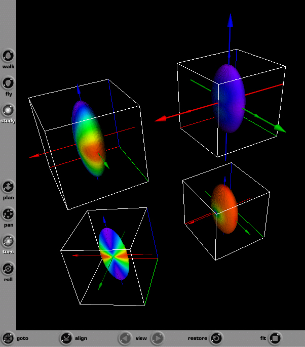
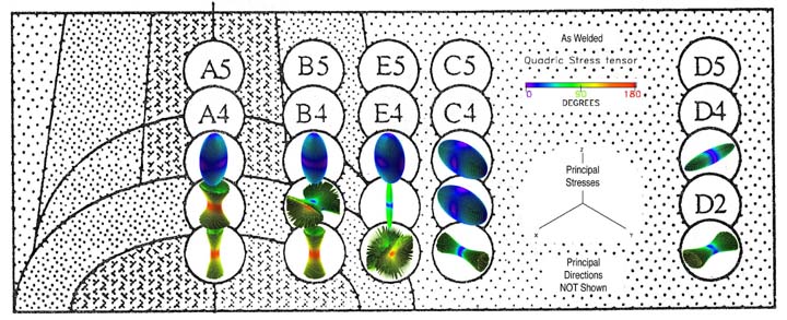
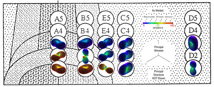
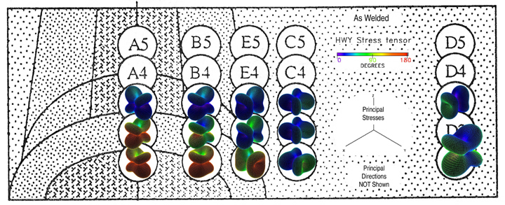
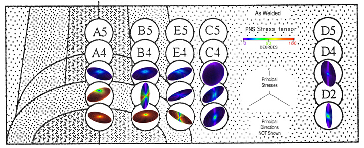
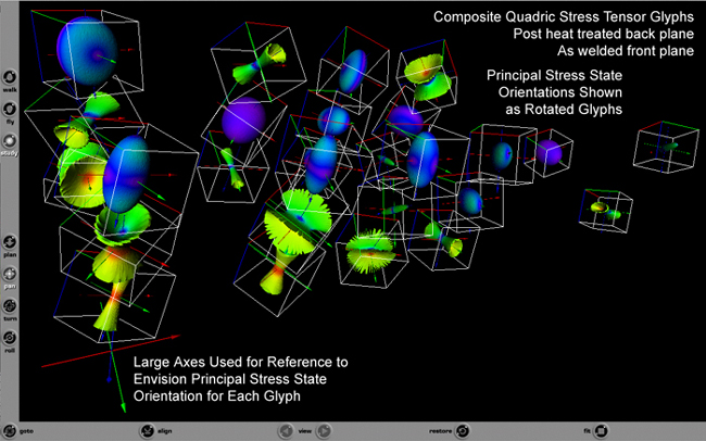
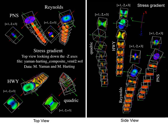
Figure 49. Residual stress profiles,
VRML-1 and
VRML-2, caused by shot peening near the surface of a Titanium alloy.
Δσij / ΔXk (32)
σij,k (33)
σkj,k (34)
Envisioning Fourth-Order Stiffness Tensors, Cijkl
This relationship is called generalized Hooke's law. This equation is a tensor
equation and can not be written in matrix notation unless using contracted
Voigt notation. This contracted format is written as 6x6 matrice, however
these contract terms will not transform as tensor components. Here the
tensor format is maintain that will prove useful when envisioning physical
properties associated with mathemtical invariance of tensor equations. This
mathematic invariance can be demonstrated when each term of the tensor Eqn.
(36) is transformed as a tensor of that order and the original form of the
tensor equation remains unchanged. When Eqn. (35) is combinded with the
equations of motion, the result is another tensor equation called the
Christoffel's equations of motion, Eqn. (36). A complete development of
Christoffel's equations can be studied at: Introduction to
Mechanical Behavior of Anisotropic Materials: Geometric Representations of
Elastic Anisotropy: All Tensor Components, Cijkl".
![]() (36)
(36)
Wavesurfaces are created using the VRML-1 and -2 file formats, that enables the
viewer to interact with and interpret complex 3D wave surface geometries as a
fourth order tensor "glyph".
Glyph geometry defined.
Depending on the user's computer configuration,
NIST has provided a
VRML Plugin and Browser Detector that the viewer can select and
install the appropriate plugin. Access details on how-to-create
these wave surfaces using PV-Wave software, Ref.[21].
Below are archived examples of the most
common crystal class symmetries.
![]() (36)
(36)
![]() (15)
(15)
and the scalar terms
![]() (37) and (38)
(37) and (38)
![]() (39)
(39)
![]() (40).
(40).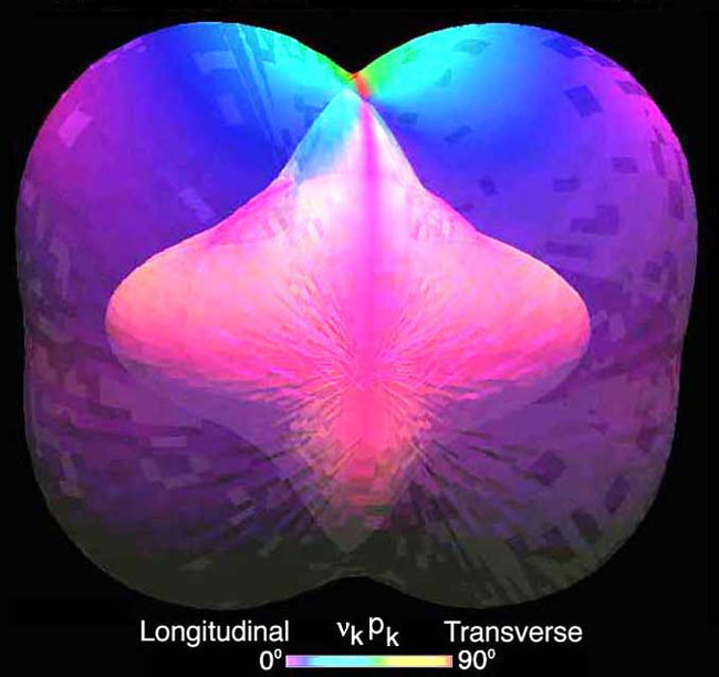
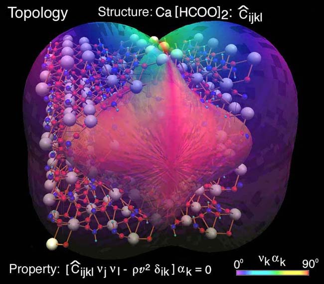
Figure 57. Linking the macro- and nano-scales. Understanding material anisotropy
of Calcium Formate.
Envisioning Sixth-Order Stress Induced Anisotropy Tensors, Cijklmn
The contents of this web site are © Copyright Ronald D. Kriz. You may
print or save an electronic copy of parts of this web site for your own
personal use. If used elsewhere in published or unpublished form please
cite as, "private communication, R.D. Kriz" and include link to this web
address. Permission must be sought for any other use.
Send comments to: rkriz@vt.edu
Ronald D. Kriz, Short Bio
Engineering Science and Mechanics
College of Engineering
Virginia Tech
Blacksburg, Virginia 24061
Revised 08/09/06
Original: http://www.sv.vt.edu/classes/ESM4714/methods/EEG.html